Iolite 3 has arrived! (and we've moved...)

We've been working for some time on our major upgrade to iolite 3 and now it's finally here.
The new version has an entirely reworked interface where we've worked hard on making things more intuitive and providing a smoother workflow. In addition there are some great new features such as full support for split-stream data acquisition (i.e., import and synchronisation of data from two different mass spectrometers).
And now that the main update is done we're hard at work on some great new features such as data reduction schemes for solution-mode trace elements work and laser U-Pb dating of common-Pb rich minerals.

As part of the upgrade to iolite 3 we've moved all of our various online support materials (i.e., the forum, blog, and online manuals) onto our new website so that everything is easily accessible in a single location.
Of course this means this blog will no longer be actively maintained, so we encourage everyone to head over to the new blog (all of the older posts on this site are also available on the new blog).

New Mass Spec Sync feature demo

We've been working hard on iolite 3, and one of the features we're excited about is the new Mass Spec Sync feature. We've put together a quick (3 min) demonstration of how it works in the video below... and it gives you a sneak peak at the new iolite 3 interface... well, parts of it anyway.

If you have any questions about this feature, or the Iolite 2014 Workshop, please head on over to the forum and ask away!

The Iolite Team

Iolite Workshop 2014

7th and 8th of June

(Photo Credit: John Creech)

We will be holding an Iolite workshop this year in conjunction with the Goldschmidt conference in Sacramento, California. It will have a very similar format to last year's workshop, but will include all the new features that will come with Iolite v3. We will also include sessions on our upcoming U-Pb DRS, our new 3D imaging module, as well as any other features developed before then. We start from the very basics, but by the end of the workshop, you should be able to write your own data reduction schemes, and know how Iolite stores all your data, and propagates errors.

So if you're a new Iolite user, or an experienced Ioliter but would like to get the latest on Iolite's ongoing development, come along and check it out. It's also a great chance to speak with the Iolite team to get specific answers, or to discuss possible features in upcoming releases.

Seats will be limited to 50 participants, so get in early to make sure you don't miss out! (Last year we were at capacity).

So, the details are:
Place: Sacramento Convention Center, 1400 J Street, Sacramento
Dates: 7 and 8th of June, 2014, 9am to 5pm (or earlier on Sunday to allow attendees to make it to the Goldschmidt icebreaker)
Cost: $300 for both days. $200 for students

What to bring: A laptop with a screen resolution greater than 1200 * 800, a power cable and mouse, IgorPro already installed (a trial version can be used for the workshop as long as it has not expired). Pens and paper.

Themes to be covered will include the following:

• An introduction to the new Iolite 3 interface and data reduction flow
• How to install and use Iolite
• Loading and checking mass spec data in Iolite
• Various data reduction examples (including trace elements and U-Pb geochronology)
• How to use Iolite for solution analyses
• Creating laser ablation images in Iolite
• Error propagation and estimation
• Creating and editing reference material files (i.e. how to use your own values for reference materials like NIST SRM 612 etc)
• Creating and editing your own Data Reduction Schemes

Last year, we had everyone writing Iolite code by the end of the second day! If there's anything you'd like covered, or would like more information about the topics outlined above, head over to the forum and ask away!

To register your spot in the workshop, please register via the TryBooking website.

Please note that this is an Iolite v3 workshop. Iolite v3 is a commercial version of Iolite. Workshop participants with be given a free, time-limited copy of Iolite v3 to work with during the course for those that do not already have a fully licensed version. The time-limited version will expire 1 month after the workshop.

We will send out more details regarding payment methods etc closer to the workshop date.


The Iolite Team

How To Use The New Laser Log File Importer

Here is a quick demo of the new laser log file importer:

What Iolite does so far...

As noted in the last post we're all buzzing after Goldschmidt (of course from the workshop, but also from a whole week of stimulating discussions), and we're now busy working on Iolite 3 among other things. But in the midst of all of this looking forward it occurred to us that this might be a good time to look back at what's been achieved so far. So here's a (probably incomplete) list of ways in which Iolite has been used by the community to date:

Laser ablation
Sr-isotope ratios (REE correction, e.g. perovskite)
Sr-isotope ratios (CaAr correction, e.g. carbonate)
Hf-isotope ratios
Nd-isotope ratios
Pb-isotope ratios
Trace element analysis (semi-quantitative normalisation)
Trace element analysis (internal standard normalisation)
Trace element analysis (varying internal standard normalisation)
Conventional laser mapping
Coordinate-based laser mapping (Cellspace)
Mineral-dependent laser mapping (MinMapping)
U-(Th)-Pb geochronology

Solution mode
Trace element analysis (semi-quantitative)
Al-Mg elemental ratios (mixed spike)
Relative Mg-isotope ratios
Absolute Mg-isotope ratios (double spike)
Fe-isotope ratios (double spike)
Mo-isotope ratios (double spike)
Si-isotope ratios
Hf-isotope ratios
Pt-isotope ratios (double spike)
Ni-isotope ratios
Cr-isotope ratios
U-isotope ratios (double spike)
W-isotope ratios
Cu-isotope ratios
Ca-isotope ratios

TIMS
Ba-isotope ratios
Ca-isotope ratios
Sr-isotope ratios
Cr-isotope ratios

If you have used Iolite for some other purpose, feel free to comment, and we'll add it to the list!

Last word from the Iolite Workshop 2013

To all those who attended our Iolite Workshop 2013 in conjunction with the V.M. Goldschmidt conference, thank you for coming!
It was great to see some really interested users from a range of backgrounds and with a variety of exposure to Iolite. The feedback we received was fantastic and we're loaded with new ideas. We're working towards getting some of these things ready for the next release (like the ability to synchronise data from two mass spectrometers), while other bigger changes will be incorporated into Iolite 3. We haven't mentioned much yet on the blog about Iolite 3, but as the name suggests it will be a major upgrade – mainly to the user interface and workflow of Iolite – and more details will follow in future blog posts as development progresses.

Despite the heat (the aircon wasn't working from the start of the workshop) and the timestamp issues (we've spoken to the relevant mass spec company), participants were enthusiastic and engaged. We also gained a lot from the discussion of open data and increasing data half-lives.

We have lots of big things planned for Iolite, and we also appreciate that if researchers are investing time in learning to use our software we have to ensure Iolite sticks around and remains relevant, so we're working hard on keeping Iolite moving forward.

So a big thank you to all the participants, and to those who couldn't make it this time, there will be more.

The Iolite Team

Customising Iolite, Part II

In our previous post, we discussed some basic ways to customise Iolite. Continuing on from there, we'll look at how to set up the Traces Window so that it displays your favourite channels, with your preferred zoom levels, each time you crunch your data.

It's quite common that if you're analysing similar samples regularly, such as zircons, you might use the same channels over and over to select your baselines, reference materials and unknowns. Every time you'll have to choose your favourite channels from the list and set up the axis limits. However, if you use one of the more common DRS, you may have noticed these buttons in the top left of the Traces Window:

By default, if you're using the Trace_Elements DRS and click on the View Baselines button, it will automatically try to show the Ca43, Sr88, Ba138 and a bunch of other channels. Ca43 will be the Primary Channel, and the axis will be set to display between 0 and 15000 CPS. The View Intermediates button does something similar, but with intermediate channels. You can change what channels are displayed, what order they are displayed in, and what zoom levels to use.

The setup for these buttons is stored in the DRS. A lot of the DRS we distribute with Iolite don't have the code in there by default. But you can easily add it by copying and pasting the code below into the bottom of your DRS beneath all the other code, and customise it to suit your needs. Here's what the codes looks like:

Function AutoBaselines(buttonstructure) //Setup Auto Baselines button --- This is based off a button, so has button structure for the next few lines
STRUCT WMButtonAction&buttonstructure
if( buttonstructure.eventCode != 2 )
return 0  // we only want to handle mouse up (i.e. a released click), so exit if this wasn't what caused it
endif  //otherwise, respond to the popup click
ClearAllTraces()

 AutoTrace(0, "Ca43", 0, 15000, extraflag = "Primary")
AutoTrace(1, "Sr88", 0, 5000)
AutoTrace(2, "Ba138", 0, 4000)
AutoTrace(3, "Pb208", 0, 5000)
AutoTrace(4, "Th232", 0, 2000)
AutoTrace(5, "U238", 0, 800, extraflag = "Right")
AutoTrace(6, "Ce140", 0, 500, extraflag = "Hidden")

End           //end of code


You can ignore all the code up to where it first says "AutoTrace(.......)". This is where you can customise it. Let's look at what the stuff between the brackets means:

AutoTrace(TraceNumber, "ChannelName", AxisMinimum, AxisMaximum)

TraceNumber is just the order of the traces, and should be a number, as in the example.
"ChannelName" is the name of the channel you want to display. Don't forget the quotation marks!
AxisMinimum and AxisMaximum are the minimum and maximum values for the axis this trace will be plotted on.

There are also a few extra flags you can add between the brackets (see the Ca43, U238, and Ce140 traces in the example above). If you're going to use them, make sure you include the "extraflag = " part too!

Setting up the View Intermediates button is exactly the same. The only difference is in the Function name. Here's an example:

Function AutoIntermediates(buttonstructure) //Setup the View Intermediates button --- This is based off a button, so has button structure for the next few lines
STRUCT WMButtonAction&buttonstructure
if( buttonstructure.eventCode != 2 )
return 0  // we only want to handle mouse up (i.e. a released click), so exit if this wasn't what caused it
endif  //otherwise, respond to the popup click
ClearAllTraces()

AutoTrace(0, "Ca43_CPS", 0, 0)
AutoTrace(1, "Sr88_v_Ca43", 0, 0)
AutoTrace(2, "Ba138_v_Ca43", 0, 0)
AutoTrace(3, "Pb208_v_Ca43", 0, 0, extraflag = "Primary")
AutoTrace(4, "Th232_v_Ca43", 0, 0)
AutoTrace(5, "U238_v_Ca43", 0, 0, extraflag = "Right")
AutoTrace(6, "Ce140_v_Ca43", 0, 0, extraflag = "Hidden")

End      //End setup function

Notice the different function name (this time it's "AutoIntermediates") and that the channel names are intermediate channels, but they don't have to be! You can use input or intermediate channels in whatever combination you like. The setup for the AutoTrace lines is exactly the same, but you'll notice that in this example, AxisMinimum and AxisMaximum all set to 0. If they're both set to 0, Iolite will automatically set the zoom levels.

After you've pasted the code into your DRS, make sure you save the DRS file by going to File -> Save Procedure. And then whenever you click on the View Baselines or View Intermediates buttons in the Traces Window, it will automatically set up the Traces Window with your favourite settings.

If you have any troubles with setting up these buttons, feel free to create a new topic on the Iolite forum, or add a comment to this post.


The Iolite Team

Customising Iolite - Part 1

There are plenty of ways to customise Iolite. We're going to break them up into three main categories: basics, viewing, and DRS specific. So let's start with the basics.

If you haven't already noticed, in the Iolite menu at the top, there's an item called "Modify Iolite's default settings". Selecting this item opens a panel showing the basic settings that you can change. Note that any changes you make here will usually take effect for the next experiment you start, not the current one.

Lets go through what each of these mean.

Show info panel on main control window: If this option is checked, a small info panel will appear at the bottom of the Main Control Window. This panel shows information about any cursors currently placed in the window. By default, you won't have any cursors in the window, so this is usually left unchecked.

Show sample labels: Checking this option will show the filename from which the data was loaded at the first point of the data. This will be printed in blue and be vertically aligned. This is the same as checking the box in top left of the Main Control Window, and chooses whether this box is checked by default.

Show integration labels: Each integration can have its own "annotation" or label. This can be entered manually or automatically if you have a laser log file or use one of the other automatic integration methods. Checking this box makes these labels appear by default.

Use native GUI appearance: Igor Pro allows programmers to set whether the buttons and other user interface items, like drop-down menus etc, will take the default Igor appears (rather square looking with flat colours) or use the system OS appearance. For example, if you're using Igor Pro on a Mac running OS 10.7, the buttons will appear more 3D and have rounded corners etc. This option may sound rather aesthetic but if you're experiencing slow performance while using Iolite, try unchecking this option.

Stats method to use for baselines: You can select the default outlier rejection to be used for calculating mean of each baseline integration using this option. Open the drop-down menu to see all of the choices. The default is currently "mean with 2 S.D. outlier reject" but as this will reject the outside ~3% of points even if they're normally distributed, I would suggest setting the default to "mean with 3 S.D. outlier reject". Remember, this the default that will be used when you start a new experiment. You can change the stats method for individual experiments by clicking on the "Edit Settings" button in the Main Control Window.

Stats method for normal integrations: This is the same as for baselines but will select the method for all other integration types, i.e. reference materials and unknowns. 

Import file type: Use this option to select the file type you most often import. For example, if you mostly reduce Agilent data using Iolite, set this option to Agilent.csv. For all new experiments, Agilent.csv will be the default file type in the import options window that appears when you click the Import Data button.

Import single file or folder: Similar to the above option, this selects whether you want to open individual files, or entire folders, by default.

Colour scheme to use in images: when you first create an image, Iolite will look for your default colour scheme and use that to colour your images. You can set this default colour scheme here.

Preferred import folder: Use this option to select the folder you most often import files from. For example, if you have a folder you store all your raw data in called "My Mass Spec Data", use this option to select that folder and when you next import data, Iolite will automatically go to your "My Mass Spec Data" folder to allow you to select your raw data file.

Overwrite existing integrations: This option comes into play when you use one of the automatic integrations methods, such as a laser log file. If you have already selected integrations in an integration type (e.g. G_NIST612), when you try to automatically add integrations to the same integration type, Iolite asks you whether you want to delete the existing integrations and replace them with the new ones you've just defined, or whether you want to keep them and add the new ones as well. If you're adding a lot of integrations automatically, you can be asked this question quite a few times, so use this option to set whichever you'd like to be the default action. You will still be asked to confirm, but your preferred option will be the default.

This is how to change some of the basic settings in Iolite. In the next blog post, we'll show you how to set the Traces Window up so that it shows your favourite channels, with your preferred zoom settings too.

If you have any suggestions for default settings that you wish you could change, please let us know in the comments, or feel free to start a new topic on the forum.

The Iolite Team

Determining the start time of spot analyses for downhole fractionation correction in the UPb DRS

As with the last post, this is a follow-up to a question posted on the Iolite forum, this time by Jiri Slama (the forum thread can be found here). To summarise, he has previously used a raster pattern when measuring U-Pb ages in zircons, and wanted to know whether there is a best practice when using spot analyses. In particular, he asked how the start time of each analysis (i.e., when the laser shutter opens and ablation commences) is determined, and whether it is necessary to strictly maintain the same timing for baselines and analyses within a session in order for this "time=0" to be consistent between each spot analysis.


First of all, I think this is a great question, as the correct determination of time=0 is critical to properly treating the downhole fractionation in each analysis, regardless of the method used. If a spot analysis is corrected based on a start time that is inaccurate this will introduce a bias in calculated ages that may well be significant.

The way we do this in Iolite is quite different from many other data reduction strategies, so I think it's worth clarifying those differences first. The most common approaches are using a linear fit, or regressing the data to the y-intercept (both assume that downhole fractionation is linear). In both cases a line is fit through the data (either from each spot analysis individually, or by assuming that all analyses are identical, and thus share the same slope). This is then either used to subtract the effects of downhole fractionation to produce a "flattened" analysis, or to infer what the ratio would have been at the time the laser shutter opened (because there was no hole at this point it is assumed that downhole fractionation was zero). The former produces corrected ratios for each timeslice of data, whereas the latter yields a single value and associated uncertainty on the regression. Obviously for these methods to work it is essential that the time=0 used is consistent between analyses to avoid either over- or undercorrecting ratios. In many cases the easiest way to achieve this consistency is by structuring analyses within a session so that the duration of the different components of each analysis (i.e., baselines, spot analysis, and washout) are always the same. It is then always straightforward to select and compare equivalent timeslices from each analysis.

In Iolite there are a couple of differences from the above - the first is that there are methods of correcting downhole fractionation (e.g., an exponential curve) that do not correct the data back to time=0 in the same way as when using a linear fit. This can have an influence on the apparent ages at intermediate steps of data reduction (there's a blog post about that here), but does not have an impact on final ages. And most relevant to this post, the consistent selecting of time=0 is still every bit as important as when using linear fits. Although having said that, it doesn't matter if time=0 perfectly coincides with the moment that ablation commenced, provided that it is the same for every single analysis (this is also true for linear fitting where all analyses are assumed to have identical slope).

The second difference is the big one - in Iolite there are different options available for the way in which time=0 is determined. These different methods have pros and cons, and it's important to confirm that the method used is producing the correct outcome. The big advantage of this flexibility of approach is that it allows for freedom in how data are both acquired and reduced. For example, if analytical conditions are stable it may be preferable to acquire longer baselines every 5 analyses, instead of a short baseline prior to every spot analysis. Likewise, if during data reduction it becomes obvious that the early portion of an analysis is rubbish there is no problem with only selecting the latter range of data.

Regardless of what method is used to determine time=0, there is a specific channel in Iolite that stores information about how long the laser shutter has been open for. It is called "Beam_Seconds" and can be found in the intermediate channels list once it has been calculated (if you make changes it will be recalculated when you crunch data). Below is an image showing Beam_Seconds versus (red) overlaid on 238U signal intensity (grey), plotted against time on the x axis.

I realise that at first glance this may look a bit strange, but you can see that it shows the time that has elapsed since the laser began ablating steadily increasing until the beginning of the next analysis, at which point it is reset back to zero. It probably makes a lot more sense once it is converted into an x-y plot of Beam_Seconds (x-axis) versus 238U intensity (y-axis):

Now you can more clearly see each analysis and its subsequent washout down to the baseline. It is hopefully also obvious that by using Beam_Seconds it is easy to compare different analyses in relation to the time since the laser started firing (which we assume directly relates to how deep the laser pit is).

So that's how we keep track of Beam_Seconds in Iolite, now the next thing is how it is determined. There are three different methods, with a 4th one in the pipeline:

"Cutoff Threshold" - This is the easiest one to explain: every time the intensity of the index channel increases over the threshold set using "BeamSeconds Sensitivity" the Beam_Seconds channel is reset to zero. This works really well in cases where there is not a sharp wash-in of the signal. But it should be noted that the value selected should be as low as possible (different thresholds can be tested until the Beam_Seconds wave produced the correct result), otherwise there may be a significant difference in the trip point between grains with high and low abundances of the index isotope.

"Gaps in data" - In the vast majority of cases this will work off the time since the beginning of each data file. Thus, in cases where each analysis is acquired in a separate file this will allow you to set a specific elapsed time (in seconds, set using the "BeamSeconds Sensitivity" variable) since the start of each file as the trip point for resetting Beam_Seconds.

"Rate of change" - This is the clever one, it uses a snappy little algorithm based on the rate of change of the signal to determine the time at which the laser starts firing (this is where the logarithm of the signal increases most rapidly). It does the best job of consistently finding the same point in each analysis, despite differences in signal intensity, but unfortunately it is also quite susceptible to noisy or spiky analyses, and is thus quite prone to failure. So, as usual, careful checking of results is important.

"Laser log file" - This one is still in the pipeline, but as the name suggests, it will use the laser shutter open events stored in the laser log file to determine when to reset Beam_Seconds.

One thing that is important to clarify is that (regardless of which of the above methods is used) the determination of Beam_Seconds is entirely independent of the masking of low signals. So even if the signal is masked up to the point at which the laser began to fire this does not necessarily mean that the Beam_Seconds wave will coincide. Similarly, the integration periods selected for each analysis are also entirely independent of Beam_Seconds. As such, editing an integration period to exclude the beginning of an analysis will have no impact on the calculation of time=0 and how downhole fractionation correction is performed).

Hopefully this provides some more detail to those not entirely sure of how these calculations are performed in Iolite, and as always if you have any questions feel free to post on the forum. Also, if you want to know more about making sure that Beam_Seconds is calculated correctly there is a blog post about that here.

Downhole corrected UPb ages and general workflow of the U-(Th)-Pb Geochronology DRS

I was recently asked on the forum to explain the downhole-corrected ages produced by the UPb DRS, and Luigi suggested that I turn my reply into a blog post – so here it is…

To give a bit of context (the original forum thread can also be found here), Luigi noticed that his downhole-corrected ratios (e.g., "DC_206_238") and their related ages were quite inaccurate, and was naturally concerned that this was affecting his results. He observed that the raw ratios were reasonably close to the accepted ratios, but that despite having significantly better uncertainties, his downhole-corrected ratios were about double what they should be, and that his final ratios and subsequent ages were nevertheless coming out with the right numbers.

And here's my reply (augmented a bit and with some pictures added):

What you're observing is perfectly ok, it's a natural consequence of the different steps of processing that the DRS uses.

The channels for ratio calculations are divided into three groups - "raw", "DC" (down-hole corrected), and "final".

Raw ratios
The raw ratios are hopefully pretty obvious - they're the observed ratio, and are generated by simply dividing one baseline-subtracted intensity (e.g., 206Pb) by another (238U). Here's an example of the raw 206/238 ratio from a single spot analysis, showing clear down-hole fractionation in the ratio as the analysis progresses:

 

Down-hole corrected ratios
The next step is obviously the one that's causing the confusion - down-hole corrected ratios are corrected for fractionation induced by drilling an increasingly deep laser pit into the sample (also referred to as LIEF, which stands for laser-induced elemental fractionation).
In the Iolite DRS, this correction is made using a model of downhole fractionation that is produced interactively by the user using the reference standard analyses (I'm assuming that if you're reading this you'll know the general concept - if not then I'd suggest reading our 2010 G-cubed paper). Now here's the punchline - the correction is typically made using an equation (in Iolite it's an exponential curve by default), and depending on the type of equation used, either the y-intercept or the asymptote will be the reference point from which the correction is made. So in the case of a linear fit the correction will be zero at the y-intercept, and increase linearly with hole depth.

A slight twist on this is the y-intercept method, which regresses the data back to its intercept with the y-axis (where downhole fractionation is assumed to be zero, or at the very least constant between the reference standard and the sample). This obviously also results in ratios being corrected down to their starting value.

The result of both of these is that the slope of the raw ratio gets flattened down to the value that was measured at the start of the ablation. This typically results in down-hole corrected ratios that are reasonably close to the accepted values.
In contrast, an exponential equation will be flattened up to the asymptote, meaning that the observed ratios will change quite a lot as they're shifted up towards the values measured at the end of the analysis, or likely even higher.

Of course this then means the down-hole corrected ratios will be much higher than the accepted values. I know that as you read that you're probably screaming in horror, but it's ok, it doesn't make any difference to the end result. The down-hole corrected ratios have been flattened, and whether they're accurate or not is not yet relevant.

Final ratios
This is where the reference standard spline is used to normalise down-hole corrected ratios to the accepted values of the reference standard. If for example the 206/238 ratio of the reference standard is twice as high as it should be then all 206/238 ratios in the session are halved to correct for this bias. Of course by using a spline any variability within the session can also be accounted for. It is this correction that also absorbs the high values potentially produced by using an exponential equation - if all of the flattened DC ratios were corrected 15% too high, then this step will bring them back down to accurate values.

So to bring it back to your specific questions - the DC ratios are "flattened", and that's all. The intention of this step of data reduction is to remove the down-hole effect that systematically affects every analysis, so the end result should be ratios that do not vary with hole depth (unless they really varied in the sample of course!).

The reason that you noticed a decrease in uncertainties relative to the raw ratios is that the effects of downhole fractionation have been removed, and that the resulting analysis has less variability (i.e., it's flat, not sloped). So it's a very good thing that the uncertainties are smaller, and a sign that the downhole correction is beneficial.

And finally, just to address the mention you made about dispersion - if a good downhole correction model is used then each analysis should be flattened, which is great. However, scatter between analyses is only minimally affected by this correction, so if you're seeing a lot of scatter in your DC ratios (or final ratios) then this is most likely real, and not something that you will be able to fix by playing with the downhole fractionation model. The variability may be due to differences in ablation characteristics between zircons (e.g., the effect you're seeing of systematically older/younger ages between 91500 and plesovice, which is very commonly observed). Or it may be due to changes in the conditions of ablation (e.g., different gas flows in different parts of the cell, different heights of the sample relative to the laser focus depth, etc.).
Note also that at least some of these causes of scatter will not be identified by the uncertainty propagation, and the only way to really get a grip on your overall uncertainty is by extended tests using a range of reference zircons.

If you have any questions about the above feel free to post questions either here or on the forum.

And we're open to suggestions for future blog posts, so if there are any other topics you'd like to know more about feel free to make a request!

Changes in the new UPb DRS ("U_Pb_Geochronology3")

There are some noteworthy improvements in the latest release of the UPb DRS (U_Pb_Geochronology3), so I thought I should post a description of what's changed.

One of the biggest changes is that flexibility has been added in which isotopes have been measured - previous versions required 206, 207, 208, 232, and 238 (with an option for 204). This meant that users (particularly those with Nu multicollectors) that had not measured all of these isotopes needed a modified version of the DRS. The DRS is now able to run with any combination of masses, with the only restriction being that 206Pb and 238U must be included.

Another change has been to improve the DRS' ability to identify the names of the different masses measured, regardless of their input channel name. Again, this increased flexibility will hopefully mean that fewer users need to modify the DRS to get it to work with data from their machine (that said, because of complex collector arrays and the complications of .nrf files, users of Nu multi-collectors will probably still need to use a "shortcut" file).

Next, I took up the kind offer by Joe Petrus that 207Pb/206Pb ages be moved from the VizualAge add-on to the main UPb DRS. In addition to building in the age calculation I have also modified it so that it uses a lookup table instead of an iterative calculation. I was concerned that the iterative calculation was theoretically capable of producing spurious ages, whereas the lookup table should be immune to this problem. For those interested, the lookup table spans ages from 1 Ma to 4600 Ma, in increments of 0.1%. The age for a given 7/6 ratio is then read from the table using linear interpolation between these increments (which means the actual accuracy of the lookup table readouts will be much much better than 0.1%). The decay constants used in generating the lookup table are 9.8485E-10 (235U) and 1.55125E-10 (238U).

In addition to those big things, there were also some minor changes/fixes:

---A minor bug in the down-hole fitting window that meant that manually adjusting the fit parameters sometimes failed has been fixed.

---The 238/235 ratio used in calculations is now a Global Variable that can be viewed and edited via the Edit Settings window (for now it's still the old accepted value of 137.88).

---The Global Variable that allowed setting the number of histogram bins has been removed to avoid clutter in the Edit Settings window (if anyone feels that it was useful I'd be happy to reinstate it, but I got the impression it wasn't being used).

And as always, any questions or discussions are welcomed on the Iolite forum...

Iolite Wiki gets a facelift

The Iolite Wiki (http://iolite.earthsci.unimelb.edu.au/wiki/doku) has a shiny new theme, and is now more readable. We've updated parts of the online manual, which we recommend is your first port of call if you're new to Iolite.

You can also find example data files and more information on the Trace_Element_IS and U-Pb geochronology DRS.

If you have any questions about the manual, or anything on the wiki, feel free to post a new topic on the forum.


The Iolite Team

More Iolite 2013 Workshop details

We've started preparing the Iolite 2013 Workshop, to be held in Florence, Italy, the weekend before the Goldschmidt Conference. Here is a brief list of some of the topics we will be covering:

• An introduction to the Iolite data reduction flow
• How to install and use Iolite
• Loading and checking mass spec data in Iolite
• Various data reduction examples (including trace elements and U-Pb geochronology)
• How to use Iolite for solution analyses
• Creating laser ablation images in Iolite
• Error propagation and estimation
• Creating and editing reference material files (i.e. how to use your own values for reference materials like NIST SRM 612 etc)
• Creating and editing your own Data Reduction Schemes

If there's anything you'd like covered, or would like more information about the topics outlined above, head over to the forum and ask away!

The Iolite Team

Iolite Workshop - Florence Italy 24 - 25th August 2013

Below are some provisional details regarding the Iolite Workshop, to be held in conjunction with the Goldschmidt Conference in Florence, August 2013. The workshop runs for two days, and is aimed at users of all levels from complete novice to programmer.

The first day is perfect for beginners and all those who would like to get a good grounding in Iolite basics, and will have participants working through example datasets on the day. The second day will look at particular applications (e.g. UPb geochronology) and advanced topics, such as creating or customising your own data reduction schemes.


DATES: 9 am - 5 pm 24th August, 2013 & 10 am - 3 pm 25th August, 2013
CLOSING DATE FOR REGISTRATION: 24 July, 2013
PARTICIPANTS: Limited to 50

BYO laptop and charger. Laptop screens should have a resolution of at least 1280 x 800 px.

NOTE: Some of these details may change over the coming months. Please check back regularly for updates.

Iolite Community Development

*** Updated with interference goodness! ***

Seeing as it's been a while since we last posted to the blog, we thought it'd be a good idea to point out that the Iolite team aren't the only ones working on Iolite. There are others who are improving Iolite by adding their own features to make their data reduction easier or better in some way. Here's just a couple of examples:

Interference Calculator

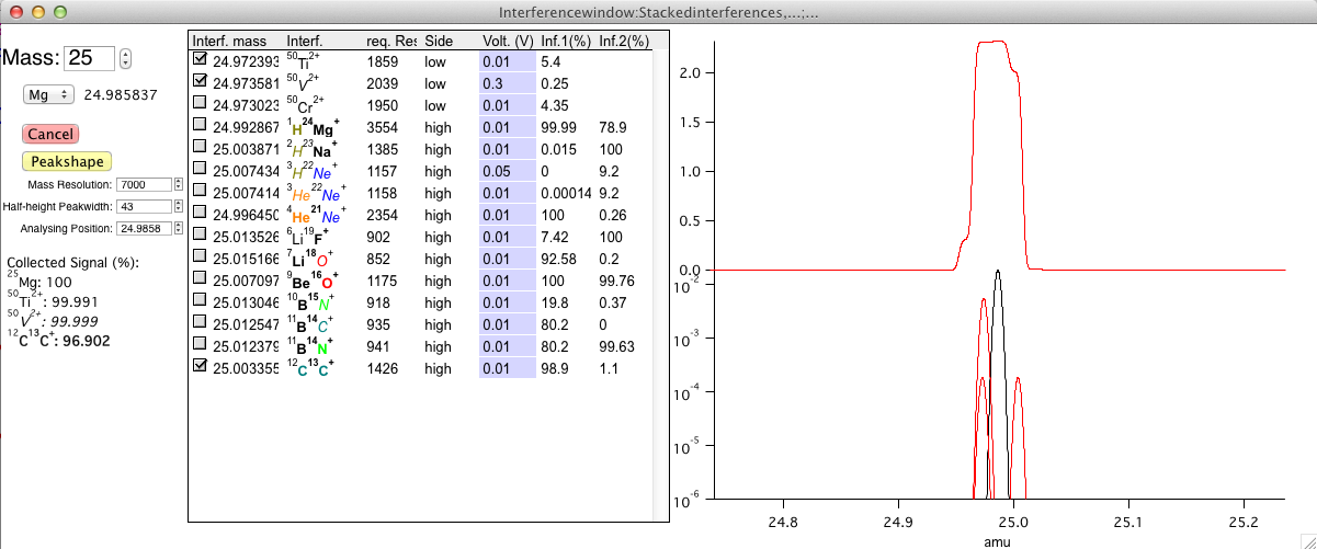
Knowing what possible interferences may affect your data can be difficult to keep track off if you analyse a variety of matrix types. Some mass spectrometers come with software that lists interferences, but what if you're processing your data away from the mass spec? What if you'd like to know what resolution you'd need to resolve an interference? Well, Martin Schiller from StarPlan in Copenhagen (with others) has written an AddOn for Iolite that will give you all sorts of information about possible interferences for a given mass. It even plots the interferences with your isotope of interest in a 'Faraday view" which is a really neat way of visualising it. Check out this post for more details.

Keep Notes with a Notebook:

If you find yourself trying lots of different approaches during your data reduction, or even if you'd just like to note down what variables you've used, Iolite has you covered thanks to the AddOn written by John Creech from Victoria University. In this post, he describes how you can add a menu item to the Iolite menu which will pop up a notebook window where you can write in all your data reduction notes. Since is stays with the experiment (that is, within the .pxp file) it's always there when you're looking at your data, even if you move the experiment between computers or even send it to your collaborators. I've started using it and I think it's very handy.

VizualAge

One of the most popular uses of Iolite is its U-Pb data reduction abilities. This has been expanded upon by Joe Petrus at Laurentian University who wrote VizualAge. If you don't know about VizualAge, you should check out the paper they published in the latest issue of Geostandards and Geoanalytical Research:

Petrus, J.A. & Kamber, B.S. (2012) VizualAge: a novel approach to laser ablation ICPMS U-Pb geochronology data reduction. Geostandards and Geoanalytical Research 36, 3 p. 247-269.

It's a pretty large paper and full of examples. Well worth a read. You can download VizualAge from Joe's webpage here.

Log Data Reader

A lot of analysts are realising how important metadata are. Instrument settings like vacuum pressure readings, lens settings and gas flows can all influence the quality of our data. The trouble is, they can be hard to keep track of, even if they are recorded in a human readable format. One step towards being able to evaluate your metadata along with your measurements is the Log Data Reader AddOn written by Martin Schiller and John Creech. So far it can read Nu Plasma and Thermo log files. Check out this post for more info.

That's just the tip of the iceberg. If you have written any additional code snippets to help you while using Iolite, we encourage you to post them to the forum where others can use them, and possibly even build on them too.

Iolite: upcoming developments

Meanwhile, Chad and I are busy working on core developments for Iolite. We're looking at some pretty fundamental changes that will probably be released as Iolite version 3. This will include upgrades to raw data importers, some really nifty improvements to how time resolved data are treated by Iolite, and a whole new user interface. Iolite v3 is a little way off, but in the meantime, we'll be releasing importers for Spectro machines and the iCAP Q, and a deconvolution tool we're writing a paper on, a new laser mapping procedure (previewed at the IGC conference in Brisbane in August), along with a few other data visualisation tools, and the usual bug fixes.

Don't forget that we're hoping to run a workshop at the Goldschmidt conference in Florence Italy in 2013, which will run over one and a half days. Hopefully this will give us enough time to take users from absolute beginners to confident gurus, with plenty of example applications.

As always, if you have any questions or comments, feel free to start a new topic on the Iolite forum.


The Iolite Team

CellSpace images tutorial

The Iolite team and Ash Norris from Resonetics have been working on a new way of creating images. We take the spatial information recorded in laser log files and combine that with mass spec data to produce images of composition versus sampling position in the laser cell. This has some great advantages:
-images don't need to be of regular shape;
-image scans don't have to be sequential (so you can measure your reference materials between scans, or several times over the course of collecting an image);
-and, you can plot your laser ablation image over mapped images of your sample collected by other means, such as photomicrographs, SEM images etc.

Here's a tutorial, using an otolith (part of a fish's auditory system) to illustrate how to create a CellSpace image, and how it can be displayed over another image. You can download the example files from this page (at the bottom) to follow along. And if you're not familiar with using laser log files, you might want to visit this page first.

[Note: Aglient users may have issues synching the example laser log file and Agilent data. If so, please delete the AgilentDateFormat.txt file in the "Other Files" subfolder within your Iolite folder and try importing the example data again.]

And just to illustrate how this approach can save time, here's a figure of how the image scan lines were arranged (green lines in right-most image) over the otolith (shown without scan lines on left and center). You can see we mostly avoid the epoxy mount, saving time and reducing the amount of gunk put into the mass spec:

Unfortunately the mouse position was not captured very well by the recording software. If you have any questions, feel free to post on the forum.

Programming Basics for Iolite

We're getting a lot of users that want to customise the way Iolite processes their data, which is really exciting as it's exactly why we built Iolite in the way that we did. But we realise that there may be many more that just find getting into the programming code a little too intimidating, or that have started to take a look but would like a few more tips.

So the aim of this post is to give a really basic introduction to how to read and understand the programming code in Iolite – it's aimed at someone with no experience with programming, so hopefully it will give confidence to those people wanting to start looking at the code behind a DRS.

The first step is to find the programming code for a DRS. To do this, go to the Iolite dropdown menu and select "Edit the active data reduction scheme" (note that you need to have a DRS selected prior to doing this). If you'd like to make changes to a DRS we'd recommend making your own DRS so that you can keep the original – the easiest way to do this is by activating a DRS that you'd like to use as a template, then selecting "Create a new data reduction scheme" from the Iolite dropdown.

Once you've selected "Edit the active data reduction scheme" a window should pop up containing the programming code. The first thing you'll notice is that it's quite colourful - this is some helpful colour coding to make it easier to identify different types of things in the text.

Red text contains comments, which don't actually do anything except explain what the code is doing. You'll notice that all comments are preceded by "//", this is IgorPro's way of identifying comments in the text, so if you put "//" anywhere on a line then everything to the right of it will be ignored by IgorPro. This is of course really useful for anyone wanting to explain what lines or sections of code do. Obviously good commenting is therefore fundamental to making code that someone else can easily read and understand.

Blue text can be thought of as defining concrete things, like functions, strings, variables and waves.

Green text indicates something that will be printed, either in the history window, a popup window or on a graph. Green text is always bounded by quotation marks.

Black text is normal text, so if you write a simple equation or refer to things (e.g., a variable) that already exist then these will be black.

There are some other colours (e.g. the purple at the top of the window), but the main colours are those listed above

Another visual aid is indentation, which is a way of denoting increasingly local code. So a first level of indentation may be for all text within a function, then a further level within that may be for a loop that runs within the function, and maybe even a 3rd level of indentation (for example if there's an "if" statement within the loop).

Igor Pro has fantastic help for programming, and instead of attempting to describe things like loops and "if" statements I'd recommend using the built-in help. To do this is really simple, just right click on anything you'd like to know more about and select "Help for …..". This right-click menu also has some other great features, like the ability to insert a template for a function, which makes it much easier to use the correct syntax.

Having said that, here's a very quick summary of the main objects you'll want to use:

String = stores text
Variable = stores a number
Wave = stores a list of numbers (or text). Waves can be thought of as a single column in a table, or a line graph. Things can get pretty complicated once waves are involved, but we've done our best to keep things simple in the DRS code, and in most cases you can operate with a wave in a very similar fashion to a variable.

It's also important to think about the order that things are laid out. When Igor Pro executes the code it runs down the code one line at a time, so things have to be laid out vertically in the order that you want them to happen (although this simple flow may look more complicated once things like loops are involved). For a given line equations are read using normal mathematical hierarchy, regardless of the order things are laid out in, so brackets will be multiplication before addition, etc.

Some programming languages are case sensitive, so a variable called "Bob" would be different to another called "bob", but Igor Pro isn't like that. You can vary between upper and lower case in the code and it generally won't make any difference. Similarly, the code isn't sensitive to spaces or blank lines, so both "X = 2 + 5" and "X= 2+5" will give the same answer (an exception to both of these things is green text - it's sensitive to both capitals and spaces).

Finally, it's handy to know that things need to be defined prior to using them. For example, if you want to store a number you can do this in a "variable", but you'll need to let Igor Pro know that you'd like to make a variable and what name it should have.

 

In a similar way, instead of creating something, you could just make a connection to something that already exists. For example, if you want to perform calculations on a wave that already exists you would need to give it a label in the function, in combination with telling Igor Pro where it's located (there's an Iolite function called "IoliteDFPath" for making the location part easy).

So, hopefully the above basic bits and pieces will help a few more people venture into the DRS code, even if it's just to have a look around. And of course there is a huge amount of detail not covered here, so if you have any questions, whether very basic or more advanced, feel free to ask us on the forum and we'll do our best to help.

Happy programming!

How to add more globals to a DRS

This is just a quick tutorial to show you how to add more global variables or global strings to a DRS. These globals are useful because they're acessible via the Edit Settings window, which means that people not comfortable with the code can quickly and easily view and modify them (e.g., the "ReferenceStandard" global string). These globals are given a default setting in the header of the DRS, which is used every time a new experiment is opened. If a user decides that they don't want to change the setting in the experiment they're working in then they do this via the "Edit Settings" window.

Below is an image of the header text in the Trace_Elements DRS.

To add a new global is pretty straightforward. First, you need to make a new line in the DRS header - the easiest way to do this is to copy an existing line of the header. Pick a GlobalVariable if you want to store a number, or GlobalString if you want to store text (in most cases you'll want to use a variable).
Put the newly copied line directly beneath the line that says "//**** Any global strings or variables you wish to use in addition to those above can be placed here", like this:

 

Now change the name to what you'd like to use (make sure it doesn't start with a number, isn't more than 30 characters long, and contains no spaces or special characters), and input your default value (or string):

Now we're done with the header text, and for the next step you'll need to look a little lower in the DRS for these lines:

 

All you need to do here is add your item to the "NVar" list if it's a GlobalVariable, or the "SVar" list if it's a Global String. Make sure you add a comma prior to your item, and that the name is identical to what you put in the line above (copy and paste is the best way to ensure this). Here's my example added to the list of variables:

Now you're all done. To use the global variable within the DRS just use it like a normal variable, e.g.:

Just note that for the change to take effect in any existing experiments you have you'll need to go to the Iolite menu and choose "Update old experiment" so that the new global gets detected by the system.
And remember, if you want to change the setting for your global, you should do this via the Edit Settings window. The header of the DRS stores the default value, which will only be read in at the beginning of a new experiment.

If you have any questions then just post a question on the forum.

Uncertainty propagation - how it works

We've had a bit of interest in propagation of uncertainties in Iolite, so I thought I'd try to do two things in this post and the next.

In this post, I'll have a go at describing our protocol for propagating uncertainties. There is a description of the method in Paton et al. (2010), but I'll give a more detailed description here with more pictures in the hope that it may further clarify it.

Then I'll follow this up in the next post by describing how to implement the protocols. Many people may not realise it, but the functions in Iolite are free for anyone to plug into their own DRS, so I'll outline how to do this, and a few things to keep an eye out for in the process.

Using splines in a DRS

In this post I'm going to give a description of how someone making or modifying a DRS can take advantage of the DRS support functions included in Iolite for working with splines. I'll use the existing "Sr_isotopes_REE" DRS as an example - it's distributed with Iolite, which should make life easy for anyone that wants to use it as a template.
The below image is all of the lines of code required – thanks to Iolite's built in DRS support functions things are kept pretty short and simple…

Before I start on the nitty gritty, there's one important detail that I think is important to understand about splines. They are made and updated by the underlying Iolite code, not the DRS. It is possible to prompt Iolite to update splines, but you won't actually be making them in the DRS. Instead, the aim in the DRS is to implement splines that already exist.

So, presumably if you're at the stage where you're trying to use splines you know the basics of editing a DRS, so I'll skip to the particulars. Firstly, you need to make sure that the wave you're interested in has a spline. In order to be splined, your wave has to be in a list of channels, so make sure that you've added it to one, e.g.:

One other thing is worth noting, and that is that only pre-defined standards (i.e., those that pop up in the list of integrations) and the Baseline_1 integration type will be splined. Output_1, and any integration types you make yourself will never get a spline.
Now, to check whether the spline you're interested in exists, you should use the function:

A couple of things are worth noting about the above function. Firstly, it looks only at the integration type that you specify, so it will not consider other integration types (in the above example I've used the Global String from the header of the DRS called ReferenceStandard, but you could put something else in there. like "G_NIST612").
The first thing that the function does is check whether the spline exists. If it doesn't then it will stop the DRS and report in the history window to let you know what happened. If this happens, everything above that line in the DRS will have been done as per usual, but nothing below that point will have been calculated.
If the spline does exist then the function will try to make sure that all other splines for that integration type are properly built and ready to use.

Ok, now that we know the spline we're interested in exists, we need to make it accessible for use in the DRS. The reason for this is that splines can have a variable number of points, depending on what type of spline they are, and the spacing of the points in the wave will not match the spacing of the Index_Time wave. The following function is used to interpolate the spline onto the Index_Time wave, after which it can be used like any other wave in the DRS:

As with the MakeIoliteWave function, you can choose whatever name for the wave that you feel is appropriate("StdSpline_Sr87_86" in this case), just be sure to keep their length <20 characters, as longer than this can potentially cause bugs. Now you have the same spline that you would see in the graph display (e.g., the main control window) available as a regular wave. Assuming that you want to normalise using the spline, the next step is to get a value for your reference standard. You can just hardwire in a value, but if you want to get more sophisticated you can also pull the value from the standard file. This way, as the reference standard is changed, your DRS will automatically use the appropriate value. To do this, you can use the following function:

This line will create a variable with the name you choose ("StdValue_Sr87_86" in this case) and get the value from the standard's text file. Just keep in mind that the name you provide needs to exactly match that in the text file ("87Sr/86Sr" in this case). Ok, now we have all the pieces required, so it's time to make a wave to hold the normalised data:

And do the actual calculation

Now the channel of normalised data is ready, so the final step is to add the new channel to the list of output channels:

All done!