We've had a bit of interest in propagation of uncertainties in Iolite, so I thought I'd try to do two things in this post and the next.
In this post, I'll have a go at describing our protocol for propagating uncertainties. There is a description of the method in Paton et al. (2010), but I'll give a more detailed description here with more pictures in the hope that it may further clarify it.
Then I'll follow this up in the next post by describing how to implement the protocols. Many people may not realise it, but the functions in Iolite are free for anyone to plug into their own DRS, so I'll outline how to do this, and a few things to keep an eye out for in the process.
1. How uncertainties are propagated
(Warning: You might want to get yourself a fresh cup of coffee, this is pretty long…)
The idea behind the uncertainty propagation in Iolite is that the can use the numerous analyses of a reference standard in our analytical session to assess the scatter between analyses, and in so doing to determine whether the internal precisions (i.e., the 2 s.e. of each integration period) are a realistic estimate of the total uncertainty.
However! The big hitch in using this approach is that we fit splines through our reference standard analyses to correct for drift within a session, and there is a risk that some (or all) of the real scatter between integration periods of the reference standard will be fitted by the spline, and as a consequence the drift-corrected values for the reference standard may have less scatter than they should. The below example shows an extreme case, where an unsmoothed cubic spline is fitted to the reference standards – unsurprisingly it does an amazing job and there is virtually no scatter left in the corrected values.


At the other extreme, we could conscientiously try to preserve all of the scatter in our reference standards by using something like a linear fit. However, we now run the risk of not correcting some of the variability that can legitimately be modelled and removed using a spline…


Clearly, something in between would be the way to go, but that leaves us in the sticky situation of not really knowing how well we've done in avoiding the real scatter while splining the systematic variability.


This is where the first big step in the uncertainty propagation kicks in. Obviously (as the first example demonstrated) we can't just use the corrected reference standards to assess scatter, so what we do instead is take each of the reference standard analyses in turn and treat it as an unknown. We can then recalculate the spline using the remaining standards and see how well they do at correcting for the "unknown". In this way, we can effectively test how well the spline does at predicting the value of a completely independent analysis, which is what we really want to know.
So here is an (admittedly rather contrived) example of this test, contrasting an unsmoothed cubic spline:


and a smoothed spline

 So during the uncertainty propagation function, we do this test (of treating each analysis as an unknown) for every one of the reference standard analyses (this is pretty heavy on the processor, but modern laptops are beasts and they don't seem to mind…), and we end up with a whole population of reference standards that were each treated as an unknown. Here is an example of such a population, plotted together with the individual uncertainties of each analysis.

After all of that, we're back to the first paragraph again, except this time we have a dataset that takes into account the real effect of the spline – if the spline is doing a terrible job then that will be reflected in our population of "unknowns", whereas if the optimal spline has been used then the scatter will have been kept to a minimum.
So now we want to assess whether the observed scatter can be explained by the internal precisions alone, or whether there is an additional source of error. And if the latter, we want to attempt to quantify that source of excess scatter and propagate it into the uncertainties.
To make this assessment, we use a statistical measure called the MSWD (mean square of weighted deviates). The reasoning behind using the MSWD is that in an ideal world of bell curves and normally distributed datasets the uncertainty on a value will describe how much scatter to expect (i.e., 95% of all values will fall within the 2 sigma error bars). With perfect uncertainties the MSWD will be 1; if the scatter cannot be explained by the error bars alone then the MSWD will be >1; and if the uncertainties are larger than they need to be then the MSWD will be less than 1.
(On a side note – the MSWD is not a good measure if you don't have many integration periods for the reference standard. This is because the MSWD distribution is asymmetric at low N, and tails to higher values. For this reason, we recommend trying to maximise the number of standard measurements in your session, either by measuring your standard more often, or by making your session longer).
So, the uncertainty propagation protocol tests our population of "unknowns", and determines the MSWD of the population based solely on the assigned internal precisions. If the MSWD is greater than 1 then it is assumed that an excess source of scatter exists. In such a case, the excess scatter is quantified as the additional error (combined in quadrature with the internal precision) required to bring the MSWD down to 1.0.
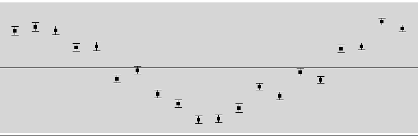
Below is an example of a group of standards treated as unknowns, showing only their internal precisions:
And the same population with error bars that include the calculated excess scatter:

Remember that this was all done using the population of standards treated as unknowns, so what we now have is the amount of excess scatter required to explain the total variability in the standards (treated as unknowns).
To then propagate the excess scatter on to samples, it is assumed that the relative uncertainty for the channel being tested (e.g., % uncertainty on the 206Pb/238U ratio) is identical for the standards and unknowns. The excess scatter is then combined in quadrature with the internal precision of every integration period for the unknowns to provide the propagated uncertainty. Because the two are being combined in quadrature, the effect of adding the excess scatter will be much more pronounced for an integration period with a very small internal precision, and may be barely detectable for integration periods with large internal precisions.
Clearly, this all hinges on the assumption that your reference standard and unknowns behave identically. If for example your standard had internal precisions that were much larger than samples (e.g. due to a lower concentration of the element of interest) then it's possible that excess scatter affecting the samples would not be detected using the reference standard analyses. Similarly, if your standards behave perfectly, but your samples are horrible, this protocol won't detect the problem with your samples. And finally, the approach only assesses scatter, so any source of systematic bias will not be detected. This is because such biases will affect the accuracy, but they won't actually generate more scatter in the data, which means that they won't have any impact on the MSWD test being used.
In this post, I'll have a go at describing our protocol for propagating uncertainties. There is a description of the method in Paton et al. (2010), but I'll give a more detailed description here with more pictures in the hope that it may further clarify it.
Then I'll follow this up in the next post by describing how to implement the protocols. Many people may not realise it, but the functions in Iolite are free for anyone to plug into their own DRS, so I'll outline how to do this, and a few things to keep an eye out for in the process.
1. How uncertainties are propagated
(Warning: You might want to get yourself a fresh cup of coffee, this is pretty long…)
The idea behind the uncertainty propagation in Iolite is that the can use the numerous analyses of a reference standard in our analytical session to assess the scatter between analyses, and in so doing to determine whether the internal precisions (i.e., the 2 s.e. of each integration period) are a realistic estimate of the total uncertainty.
However! The big hitch in using this approach is that we fit splines through our reference standard analyses to correct for drift within a session, and there is a risk that some (or all) of the real scatter between integration periods of the reference standard will be fitted by the spline, and as a consequence the drift-corrected values for the reference standard may have less scatter than they should. The below example shows an extreme case, where an unsmoothed cubic spline is fitted to the reference standards – unsurprisingly it does an amazing job and there is virtually no scatter left in the corrected values.


At the other extreme, we could conscientiously try to preserve all of the scatter in our reference standards by using something like a linear fit. However, we now run the risk of not correcting some of the variability that can legitimately be modelled and removed using a spline…


Clearly, something in between would be the way to go, but that leaves us in the sticky situation of not really knowing how well we've done in avoiding the real scatter while splining the systematic variability.


This is where the first big step in the uncertainty propagation kicks in. Obviously (as the first example demonstrated) we can't just use the corrected reference standards to assess scatter, so what we do instead is take each of the reference standard analyses in turn and treat it as an unknown. We can then recalculate the spline using the remaining standards and see how well they do at correcting for the "unknown". In this way, we can effectively test how well the spline does at predicting the value of a completely independent analysis, which is what we really want to know.
So here is an (admittedly rather contrived) example of this test, contrasting an unsmoothed cubic spline:


and a smoothed spline


After all of that, we're back to the first paragraph again, except this time we have a dataset that takes into account the real effect of the spline – if the spline is doing a terrible job then that will be reflected in our population of "unknowns", whereas if the optimal spline has been used then the scatter will have been kept to a minimum.
So now we want to assess whether the observed scatter can be explained by the internal precisions alone, or whether there is an additional source of error. And if the latter, we want to attempt to quantify that source of excess scatter and propagate it into the uncertainties.
To make this assessment, we use a statistical measure called the MSWD (mean square of weighted deviates). The reasoning behind using the MSWD is that in an ideal world of bell curves and normally distributed datasets the uncertainty on a value will describe how much scatter to expect (i.e., 95% of all values will fall within the 2 sigma error bars). With perfect uncertainties the MSWD will be 1; if the scatter cannot be explained by the error bars alone then the MSWD will be >1; and if the uncertainties are larger than they need to be then the MSWD will be less than 1.
(On a side note – the MSWD is not a good measure if you don't have many integration periods for the reference standard. This is because the MSWD distribution is asymmetric at low N, and tails to higher values. For this reason, we recommend trying to maximise the number of standard measurements in your session, either by measuring your standard more often, or by making your session longer).
So, the uncertainty propagation protocol tests our population of "unknowns", and determines the MSWD of the population based solely on the assigned internal precisions. If the MSWD is greater than 1 then it is assumed that an excess source of scatter exists. In such a case, the excess scatter is quantified as the additional error (combined in quadrature with the internal precision) required to bring the MSWD down to 1.0.
Below is an example of a group of standards treated as unknowns, showing only their internal precisions:
And the same population with error bars that include the calculated excess scatter:

Remember that this was all done using the population of standards treated as unknowns, so what we now have is the amount of excess scatter required to explain the total variability in the standards (treated as unknowns).
To then propagate the excess scatter on to samples, it is assumed that the relative uncertainty for the channel being tested (e.g., % uncertainty on the 206Pb/238U ratio) is identical for the standards and unknowns. The excess scatter is then combined in quadrature with the internal precision of every integration period for the unknowns to provide the propagated uncertainty. Because the two are being combined in quadrature, the effect of adding the excess scatter will be much more pronounced for an integration period with a very small internal precision, and may be barely detectable for integration periods with large internal precisions.
Clearly, this all hinges on the assumption that your reference standard and unknowns behave identically. If for example your standard had internal precisions that were much larger than samples (e.g. due to a lower concentration of the element of interest) then it's possible that excess scatter affecting the samples would not be detected using the reference standard analyses. Similarly, if your standards behave perfectly, but your samples are horrible, this protocol won't detect the problem with your samples. And finally, the approach only assesses scatter, so any source of systematic bias will not be detected. This is because such biases will affect the accuracy, but they won't actually generate more scatter in the data, which means that they won't have any impact on the MSWD test being used.